# XRSProcessTool User Guide
> X-ray Raman Scattering (XRS) data processing tool
> Version: 1.0 | Screenshots included
---
## 1. Introduction
XRSProcessTool is a desktop application for processing XRS experimental data from the B5 beamline. Key features:
- Load elastic-peak scan data and XRS scan data (`.nxs` format)
- Display/adjust ROIs (crystal regions of interest) on the 2D detector images
- Fit each ROI's elastic peak with a Lorentzian and reject poorly fitted crystals
- Compute momentum transfer q and filter ROIs by q range
- Interpolate and sum spectra from multiple scans and ROIs to produce the final energy-transfer spectrum
- Save results as `.txt` text files
Both single-detector (det2D) and dual-detector (lambda + minipix) modes are supported. The application starts in **dual-detector mode** by default.
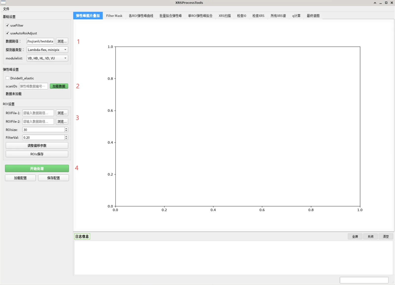
Figure 1 — Overall view of the main window
---
## 2. Startup and Layout
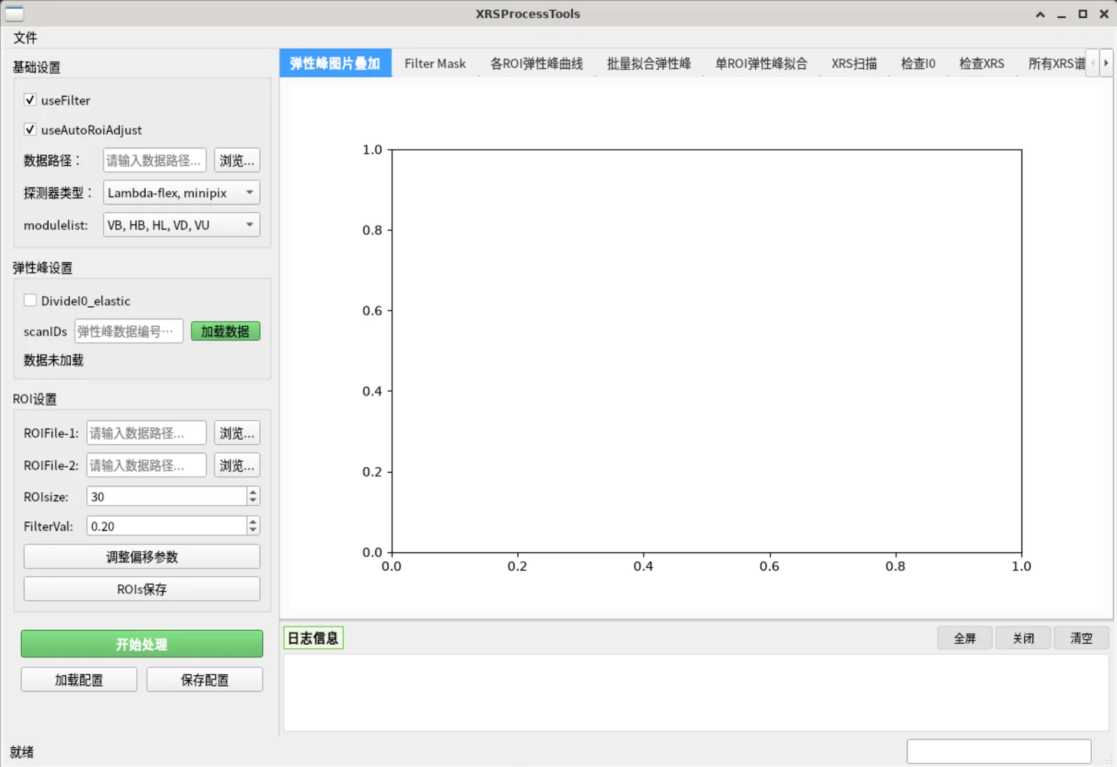
After launching `XRSProcessTool`, the main window is divided into three regions:
| Region | Description |
|--------|-------------|
| **Left panel** | Parameter settings, organized into groups (Basic Settings, Elastic Peak Settings, ROI Settings, Fitting Settings, XRS Scan Settings, Final Spectrum, etc.). Relevant groups show/hide automatically as the right-side tabs switch. |
| **Upper right** | Tab area with 11 tabs, left to right in the order of the processing workflow. |
| **Lower right** | Log panel recording operations and errors (can be cleared). |
| **Bottom status bar** | Progress bar. |
Top menu bar: **File** → Save Results / Exit, **View** → toggle the left parameter panel / log panel, **Language** → 中文 / English.
Figure 2 — Main window: parameter panel on the left, workflow tabs on the right, log panel below
---
## 3. Core Logic (read this first)
### 1. The "Process" button only processes the current tab
**"Process" will NOT run the whole workflow automatically.** It only executes the processing step for the **currently selected right-side tab**. Therefore the full workflow must be run **manually, tab by tab from left to right**.
While a tab is processing, the button turns red and shows "Processing" and is disabled; it turns green again when done.
### 2. Both panels load data by picking files directly
- **Elastic Peak Settings** → "Browse...": pick a **single** `.nxs` file (used for ROI localization and elastic peak fitting); it is read immediately and a content summary pops up
- **XRS Scan Settings** → "Browse...": pick **one or more** `.nxs` files; each file is read as it is picked. The load summary of every file goes to the **log panel**, and the status label shows the total number of loaded files plus the **scan numbers of all loaded files** (the leading digits of each file name). "Clear" removes all loaded XRS data
Both must be loaded — neither is optional. After changing parameters (I0 normalization, I0 PV, glitch removal), pick files again with "Browse..." or click "Process" on tab 5: files are re-read with the new settings, while files whose parameters did not change are not read again.
### 3. Data reuse
Loaded data stays in memory and is reused by subsequent tabs; there is no need to reload. After changing left-panel parameters, click "Process" on the corresponding tab again for the changes to take effect.
---
## 4. Data Preparation
The default data root directory is `F:/Beamlines/B5/XRSdataProcessing/data`, with the following structure:
```
data/
├── raw/ # raw scan data
│ └── 11050_scan_20260414205302_1/
│ └── 11050_scan_20260414205302_1.nxs # one folder per scan, containing the .nxs of the same name
└── processed/ # output directory for processed results
```
- **Raw data**: under `raw/`, laid out as `_scan__/.nxs`
- The **Data Path** points at the data root (e.g. `.../data`); `raw` is **not** appended to it. The file dialog opens at that directory, from which you enter `raw/` and pick the `.nxs` files; processed results are written to `processed/` under it.
- If the data path is empty, it is inferred from the selected file and filled in (a path you have already set is never overwritten).
- **ROI files**: tab-separated `.txt`, one crystal per row, columns `roi_label, x1, x2, y1, y2, x_shift, y_shift, x_expand, y_expand`. Example ROI files are bundled under `XRSProcess/ROI/` (e.g. `roi_60crystals-v3.txt`, `roi_minipix-v3-2.txt`).
> ROI file example (first few lines):
> ```
> roi_label x1 x2 y1 y2 x_shift y_shift x_expand y_expand
> VB-A1 35 66 3 31 0 0 0 0
> VB-A2 112 144 57 86 0 0 0 0
> ```
---
## 5. Full Workflow
The following steps are ordered as recommended. Main line:
> **Set basic parameters → load elastic-peak data → (tabs 0–4) ROI localization & fitting → load XRS data → (tabs 5–8) XRS checks → (tabs 9–10) q calculation & final spectrum → save results**
### Step 0: Basic Settings (Basic Settings group)
In the left "Basic Settings" group:
| Parameter | Description | Default |
|-----------|-------------|---------|
| `useFilter` | Use pixels above an intensity threshold inside the ROI box as a mask for extracting data (recommended) | ✅ |
| `useAutoRoiAdjust` | Auto-adjust ROI box position/size to the brightest pixels (recommended) | ✅ |
| Data Path | Data root directory (points to the `data` folder) | …/data |
| Detector Type | `Lambda-flex` (single) / `Lambda-flex, minipix` (dual) / `Lambda-flex-2, minipix` (dual) | dual |
| modulelist | Which modules to use: `VB,HB,HL,VD` or `VB,HB,HL,VD,VU` | includes VU |
### Step 1: Load Elastic-Peak Data (Elastic Peak Settings group)
1. Click "Browse..." and pick the elastic-peak `.nxs` file (**single file only**)
2. The file is read immediately, a content summary dialog pops up, and the status label turns green with "Data loaded: "
3. To normalize by I0, check `DivideI0_elastic` first, then click "Browse..." and pick the same file again (picking the same file twice is allowed)
### Step 2: ROI Settings (ROI Settings group)
| Control | Description |
|---------|-------------|
| `ROIFile-1` Browse | Select the main detector ROI file (required) |
| `ROIFile-2` Browse | Select the second detector (minipix) ROI file (shown in dual-detector mode, required) |
| `ROIsize` | Pixel side length of the ROI box during auto-adjust (10–100, default 30) |
| `FilterVal` | Filter threshold (0–1, default 0.2): only pixels with intensity above `FilterVal × max intensity` inside the ROI are counted |
| Adjust Offsets | Opens a dialog to set x/y offsets for each module (VB/HB/HL/VD/VU/ROI2) for alignment |
| `Save ROIs` | Export the ROI geometries adjusted in tab 0 to a new file |
---
### Tab 0: Elastic Peak Images
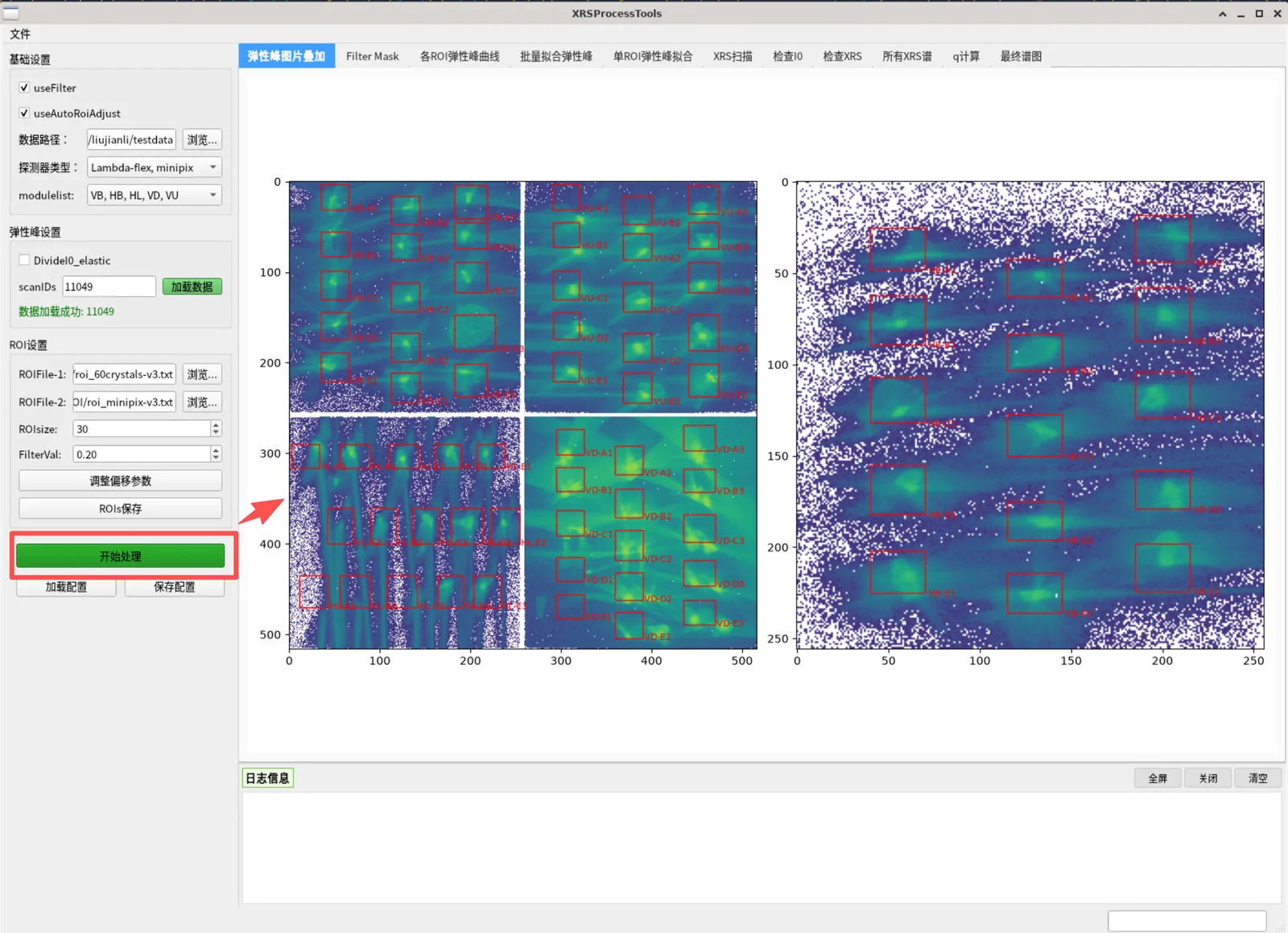
The first visualization step. Select this tab and click "Process" to show the elastic-peak scan's 2D detector image (log-scale overlay) with red ROI boxes and labels overlaid. In dual-detector mode, one image is shown per detector (lambda / minipix), side by side.
- **ROIs are interactive**: drag an ROI box directly on the image to reposition it
- After adjusting, use "Save ROIs" to export the updated ROI file
Figure 3 — Tab 0: elastic-peak 2D image with crystal ROIs overlaid
### Tab 1: Filter Mask
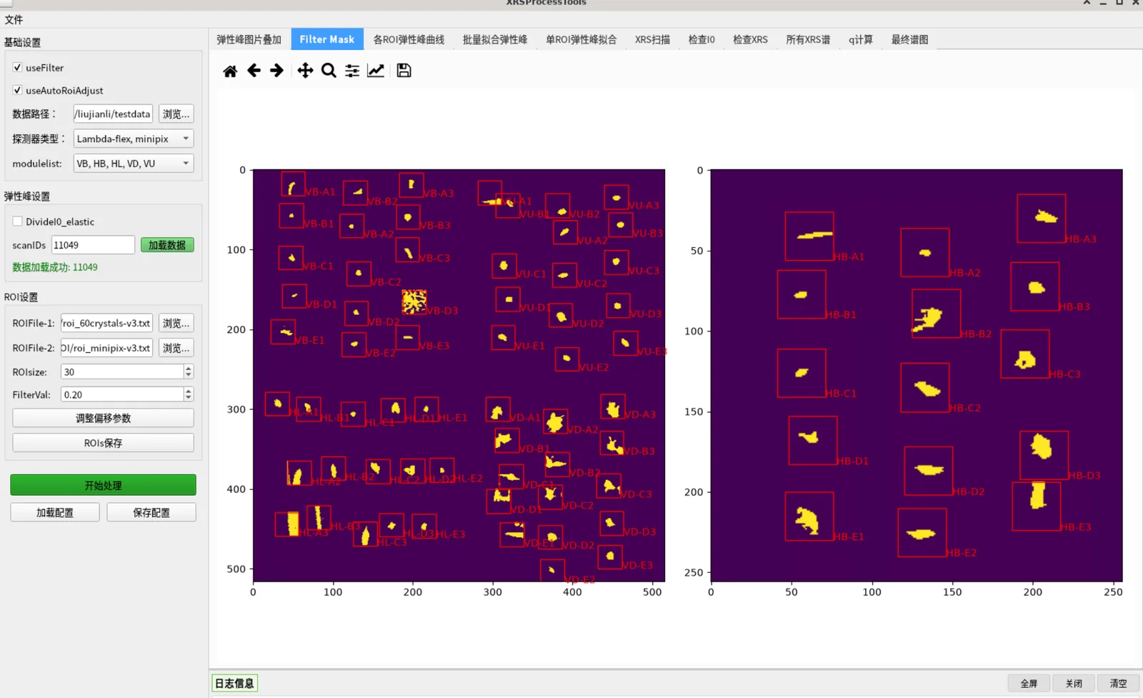
Shows the filter mask (pixels above the `FilterVal` threshold) overlaid, again with ROI boxes. If `useAutoRoiAdjust` is checked, ROIs automatically center on the brightest pixels and resize to `ROIsize`.
- Use this page to check mask quality; adjust `FilterVal` or `ROIsize` up/down and reprocess if needed
Figure 4 — Tab 1: threshold filter mask overlay
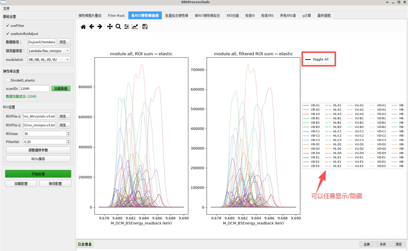
### Tab 2: ROI Elastic Peak Curves
Shows each ROI's elastic-peak curve: left plot is the raw ROI sum, right plot is the filtered sum.
Interactions:
- **Hover** a curve → highlight red and bold
- **Click a legend line** → toggle that curve show/hide
- **Click the "Toggle All" legend** → show/hide all curves at once
Figure 5 — Tab 2: elastic-peak curves of every ROI
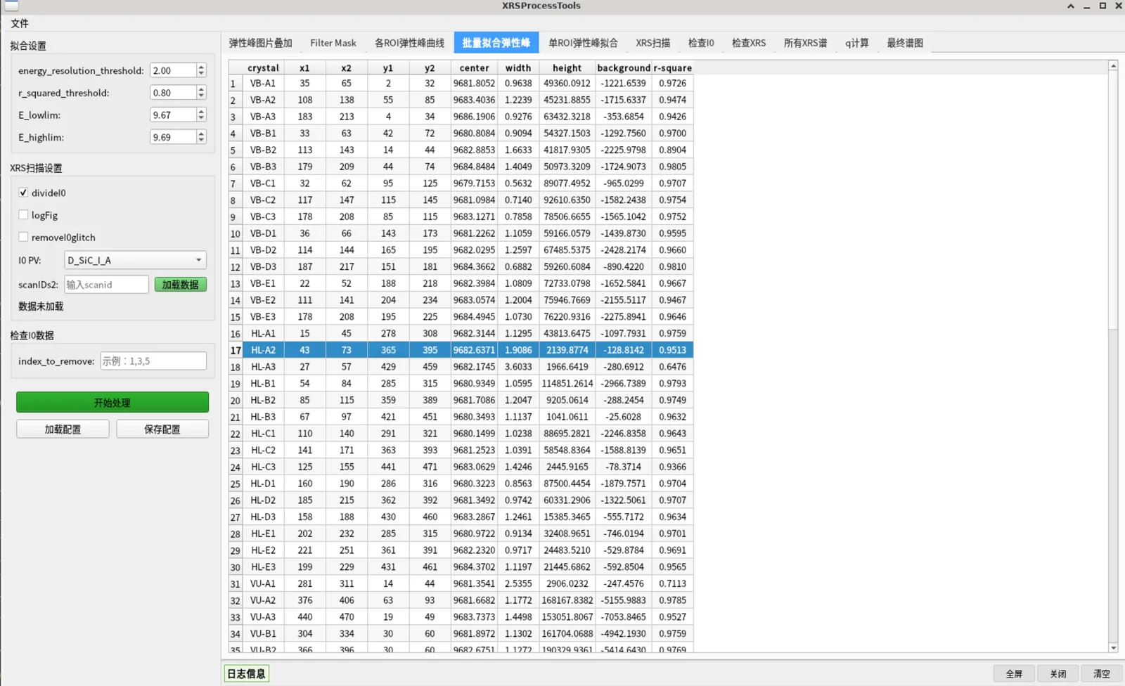
### Tab 3: Batch Fit Peaks
First set the thresholds in the "Fitting Settings" group:
| Parameter | Description | Default |
|-----------|-------------|---------|
| `energy_resolution_threshold` | Energy-resolution threshold (eV); a FWHM exceeding it is marked as a bad fit | 2.0 |
| `r_squared_threshold` | Lower bound for fit R²; below it is a bad fit | 0.8 |
| `E_lowlim` / `E_highlim` | Reasonable elastic-peak center energy range (keV) | 9.67 / 9.69 |
Select this tab and click "Process". The software fits each ROI's elastic peak with a **Lorentzian** and displays the results in a table with columns: `crystal, x1, x2, y1, y2, center[eV], width[eV], height, background, r-square, NumPixels`.
- ROIs meeting any bad-fit criterion (R² too low, center out of range, negative amplitude, FWHM too large) are added to `BadFitList` and **automatically excluded from the final spectrum**
Figure 6 — Tab 3: batch Lorentzian fitting results
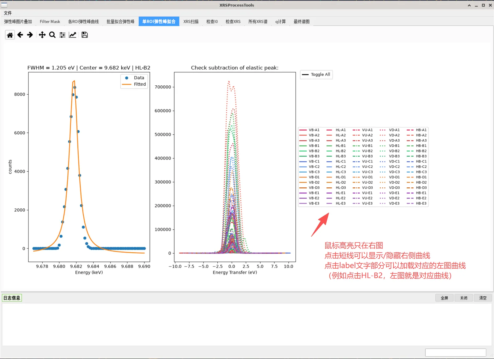
### Tab 4: Single ROI Fit
Used to inspect the fit quality of a single ROI. The left plot shows the data points and fitted curve of a crystal (with FWHM and center energy annotated); the right plot shows all ROI curves shifted so the elastic-peak energy is zero (energy-transfer view).
Figure 7 — Tab 4: single-ROI fit check and energy-transfer view
### Step 3: Load XRS Data (XRS Scan Settings group)
1. Click "Browse..." and multi-select the XRS `.nxs` files. **Each file is read as it is picked**; files can be picked over several rounds, and picking an already loaded file does not read it again
2. For every file, a load summary is written to the **log panel** (scan number, file name, 2D data shapes, number of 1D channels, I0 channel, number of glitch points removed); the status label shows "N file(s) loaded: , , …" listing every loaded file. Failed files are flagged in red
3. "Clear" empties all loaded XRS data (in-memory data and curves are reset)
4. Settings:
- `divideI0`: normalize by I0 (recommended)
- `removeI0glitch`: remove I0 glitch points (adjacent-point ratio < 0.7 treated as a glitch, replaced with the local mean)
- `I0 PV`: choose the I0 signal channel (`D_SiC_I_A` / `D_QXBPM_I_Sum` / `D_QXBPM2_I_Sum`)
- `logFig`: logarithmic plotting
After changing these, pick files again with "Browse..." or click "Process" on tab 5 to re-read with the new settings (files whose parameters did not change are not read again)
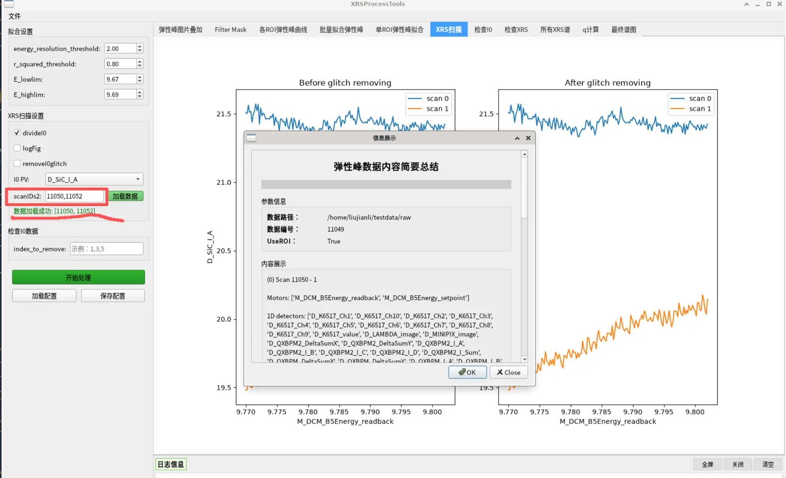
### Tab 5: XRS Scan
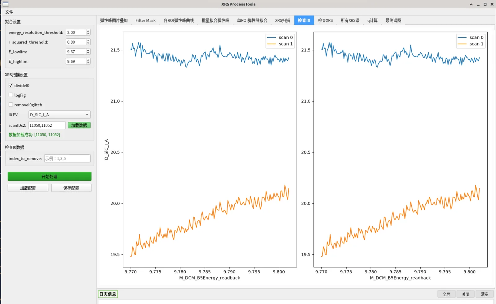
Select and click "Process" to show the I0-vs-energy curves (two subplots: before and after normalization + glitch removal), to confirm XRS data and I0 quality.
Figure 8 — Tab 5: I0 versus energy before and after normalisation and glitch removal
### Tab 6: Check I0
In the "Check I0 Data" group's `index_to_remove`, enter scan indices to exclude (e.g. `1,3,5`). After "Process", an I0 before/after removal comparison is shown, to pick out bad scans.
Figure 9 — Tab 6: I0 comparison before and after removing selected scans
### Tab 7: Check XRS
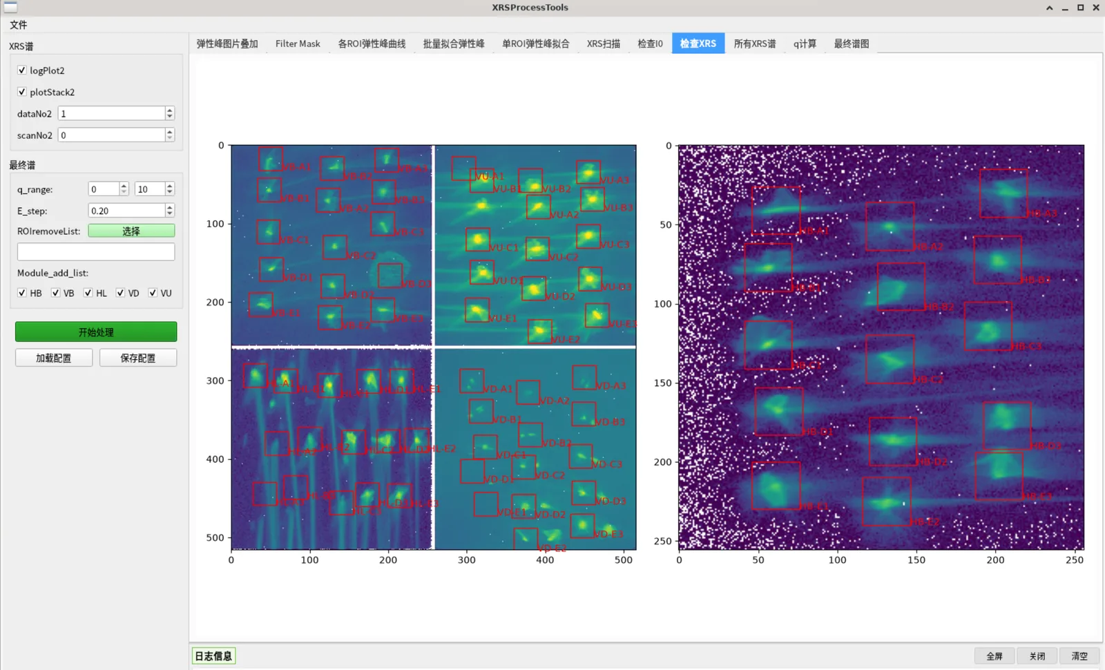
Shows the 2D stacked XRS detector image (log scale) with ROI boxes overlaid; one image per detector in dual mode. Used to check XRS image quality and ROI coverage.
Figure 10 — Tab 7: stacked 2D XRS detector image with ROI coverage
### Tab 8: All XRS Spectra
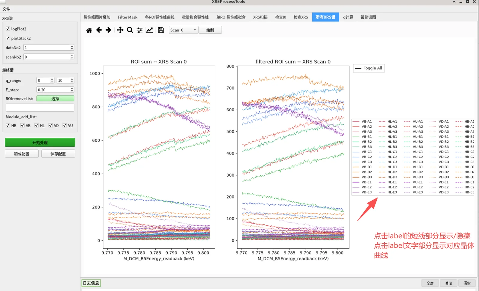
Shows the XRS spectra (raw vs filtered) for each scan and ROI.
- The top dropdown selects the scan number + a "Draw" button replots
- Hover to highlight; click a legend line to toggle visibility
- **Click a legend label** → switch to that crystal's single-spectrum view (left raw, right filtered, with scan number annotated); click "Toggle All" again to return to the overview
Figure 11 — Tab 8: XRS spectra of every scan and ROI
### Tab 9: q Calculation
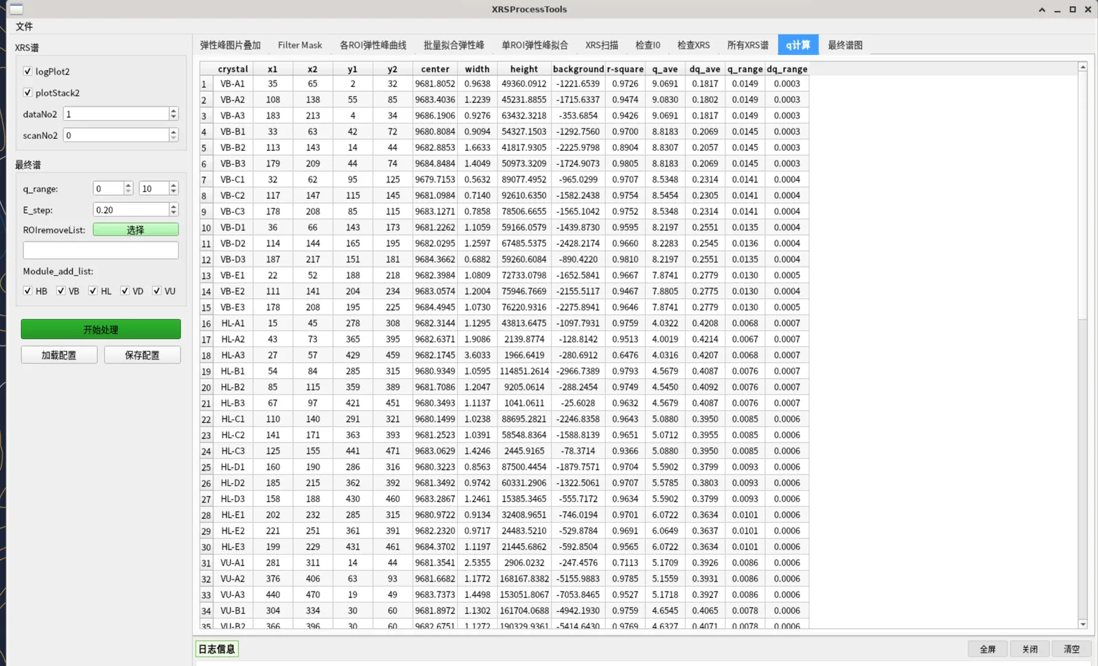
Click "Process" to compute each ROI's momentum transfer q (based on each module's fixed scattering angle and the elastic-peak energy), adding `q_ave, dq_ave, q_range, dq_range` columns to the table. This prepares the q filtering for the final spectrum.
Figure 12 — Tab 9: computed momentum transfer q
### Tab 10: Final Spectrum
In the "Final Spectrum" group, set the final-spectrum parameters:
| Parameter | Description | Default |
|-----------|-------------|---------|
| `q_range` | Only sum ROIs whose q_ave falls in this range | 0–10 |
| `E_step` | Energy interpolation step (eV) | 0.2 |
| `ROIremoveList` | Manually excluded crystals (click "Select" to pick from the crystal grid) | empty |
| `Module_add_list` | Modules participating in the sum (HB/VB/HL/VD/VU checkboxes) | all |
Click "Process" to generate the final spectrum: the top plot is the summed total spectrum, the bottom shows subplots per scan (to check the elastic-energy subtraction is correct).
Toolbar buttons:
- **Scan_N dropdown**: select scan number
- **Final Spectrum**: show only the summed total spectrum
- **Energy Transfer**: show the energy-transfer subplot of the selected scan
In the final spectrum, an ROI is excluded if it meets any of: in `ROIremoveList`, in `BadFitList`, module not selected, or q outside `q_range`.
Figure 13 — Tab 1: threshold filter mask overlay
---
## 6. Save Results
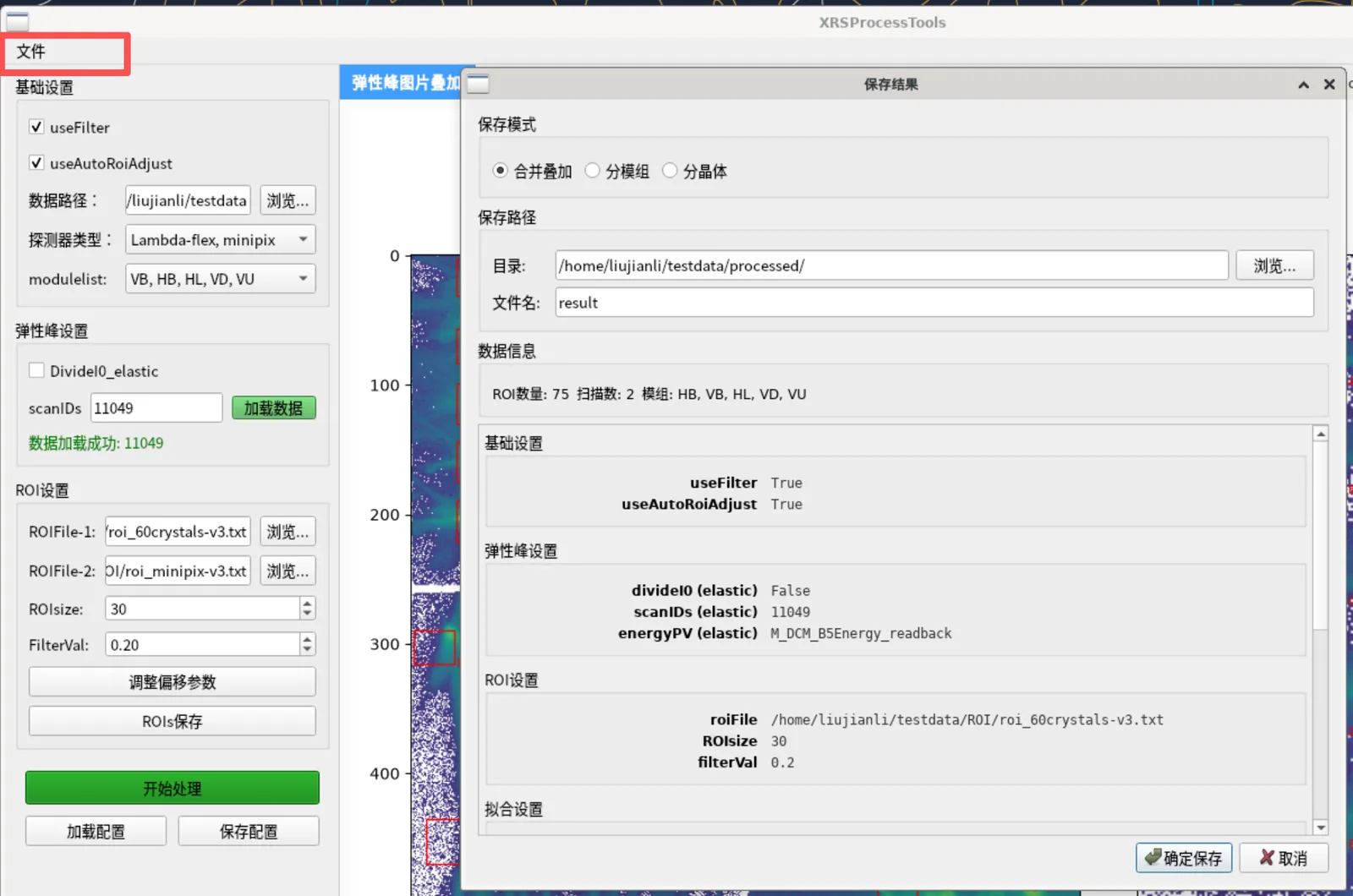
After processing, click **File → Save Results** to open the "Save Results" dialog:
1. **Save Mode** (choose one of three):
| Mode | Description | Output files |
|------|-------------|--------------|
| Merged (default) | Sum all selected ROIs into one spectrum | `_data.txt` (energy transfer + intensity) |
| By Module | One column per module, in the same file | `_data.txt` (energy + module columns) |
| By Crystal | One file per crystal + a summary | each `_data.txt` + `_all_data.txt` |
All three modes additionally output:
- `_rois.txt`: fit results (fitResult)
- `_info.txt`: a record of all processing parameters this run
2. **Save Path**: directory defaults to `/processed/`; the filename is used as the subfolder name (default `result`)
3. Confirm to save; a "Save Succeeded" prompt appears
Figure 1 — Save-results dialog: merged, per-module or per-crystal output
Output files are tab-separated text. Example (`_data.txt`):
```
Energy Transfer (eV) Intensity
90.2 20.33
90.4 18.41
…
```
---
## 7. Parameter Config Save & Load
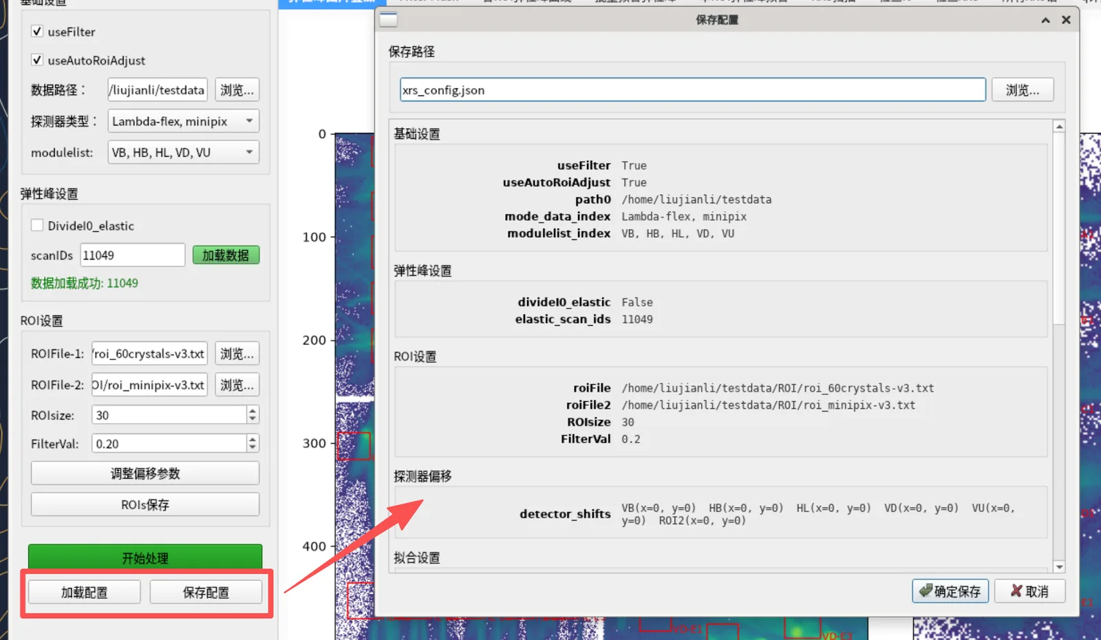
The "Load Config" and "Save Config" buttons at the bottom of the left panel save/load all parameters (including detector offsets, fitting thresholds, q range, etc.) as a `.json` file, for reuse without re-entering.
- **Save Config**: shows a parameter preview, choose a path to save as `.json`
- **Load Config**: choose a `.json` file; after validation, a preview is shown (errors in red, missing items in gray); confirm to apply to the UI
Figure 14 — Dialogs for saving and loading the parameter set
---
## 8. Quick Checklist
| Step | Action |
|------|--------|
| 1 | Basic Settings: set data path, detector type, modules |
| 2 | Elastic Peak Settings: Browse and pick a single `.nxs` (auto-read) |
| 3 | ROI Settings: choose ROIFile-1 (dual mode adds ROIFile-2), set ROIsize/FilterVal, adjust offsets as needed |
| 4 | Tab 0 → Process → check/drag ROIs, Save ROIs as needed |
| 5 | Tab 1 → Process → check mask |
| 6 | Tab 2 → Process → check per-ROI elastic peaks |
| 7 | Fitting Settings: set thresholds |
| 8 | Tab 3 → Process → view fit table, note bad fits |
| 9 | Tab 4 → Process → spot-check single-ROI fit |
| 10 | XRS Scan Settings: Browse and pick `.nxs` files (multi-select, read one by one, summaries in the log) |
| 11 | Tab 5 → Process → check I0 |
| 12 | Check I0: enter index_to_remove → Tab 6 Process |
| 13 | Tab 7 → Process → check XRS 2D image |
| 14 | Tab 8 → Process → check all XRS spectra |
| 15 | Tab 9 → Process → view q table |
| 16 | Final Spectrum: set q_range / E_step / ROIremoveList / modules |
| 17 | Tab 10 → Process → view final spectrum |
| 18 | File → Save Results → choose mode/path → OK |
---
## 9. FAQ
**Q: "Process" does nothing?**
A: Make sure a single elastic-peak file is selected and at least one XRS file has been picked (files are read as soon as you pick them; results are in the log panel), and that the correct tab is selected.
**Q: A tab shows blank?**
A: Usually a missing prerequisite step. Process the tabs left to right, ensuring previous tabs have run "Process".
**Q: Too few ROIs in the final spectrum?**
A: Check `BadFitList` (tab 3 bad fits), `ROIremoveList` (manual exclusions), `Module_add_list` (unselected modules), `q_range` (q out of range). Loosen the fit thresholds or widen the q range to include more ROIs.
**Q: Only one detector visible in dual mode?**
A: Confirm "Detector Type" is a dual-detector mode and ROIFile-2 has the minipix ROI file selected.
**Q: Chinese shows as boxes?**
A: The packaged build bundles the CJK font. Running from source requires a system CJK font (Linux: `sudo dnf install google-noto-sans-cjk-sc-fonts`).
**Q: Some parameters are wrong after loading a config?**
A: Items marked red/gray in the load dialog are erroneous or missing and will use default values; correct the source config file as prompted.
---
*This guide is updated with the software version. Contact the maintainer with any questions.*